1) Kendall's sphere of triangles
In this first workshop session, we will perform simple statistical operations in a nonlinear shape space: the set of polygons up to similarities.
The main references on the subject are:
- Shape manifolds, procrustean metrics, and complex projective spaces (1984);
- Statistical shape analysis, with applications in R (1998,2016);
- Functional and Shape Data Analysis (2016);
which are respectively Kendall's landmark paper, a classic handbook by Dryden and Mardia and a recent handbook by Srivastava and Klassen.
%matplotlib inline
import matplotlib.pyplot as plt
import plotly
# run at the start of every notebook
plotly.offline.init_notebook_mode()
# Mandatory imports...
import numpy as np
from numpy import random
import torch
from torch import tensor
from torch.nn import Parameter
# Custom modules:
from kendall_triangles import KendallTriangles # Fancy visualization
from model import Model # Optimization blackbox
from display import plot # Simple plotting routine for triangles
# Finally, emulate complex numbers with pairs of floats:
from torch_complex import rot, normalize, herm, angle, mod2, mod
A) Procustean analysis
Let us consider two non-degenerate triangles $A$ and $B$ - i.e. whose vertices are not all equal with each other. Ideally, we'd like to represent them as triplets of complex numbers... But since PyTorch 0.4 still doesn't support complex operations, we settle for 3-by-2 arrays.
A = tensor([ [-1, 0], [ 1, -.1], [ 2,.9] ])
B = tensor([ [ 1, 0], [-.5, np.sqrt(3)/2], [-.5,-np.sqrt(3)/2] ])
plt.figure()
plot(A, "red")
plot(B, "blue")
plt.axis("equal")
plt.show()

As we strive to analyse the variability between $A$ and $B$, we wish to register the former onto the latter. That is, we'd like to solve
$$ \begin{align} \arg\min_{\upsilon,\tau\in\mathbb{C}^2} &\sum_{i=1}^3 | \upsilon \cdot (A_i + \tau) - B_i|^2\\ ~=~ \arg\min_{\lambda,\theta,\tau\in\mathbb{R}\times\mathbb{R}\times\mathbb{R}^2} &\sum_{i=1}^3 | e^{\lambda+i\theta} \cdot (A_i + \tau) - B_i|^2 \end{align} $$
Such optimization problems are straightforward to solve using PyTorch:
class RigidRegistration(Model) :
"Find the optimal translation, scaling and rotation."
def __init__(self, source) :
"Defines the parameters of a rigid deformation of source."
super(Model, self).__init__()
self.x = source
self.λ = Parameter(tensor( 0. )) # log-Scale
self.θ = Parameter(tensor( 0. )) # Angle
self.τ = Parameter(tensor( [0.,0.] )) # Position
def __call__(self, x) :
"Applies the model on some point cloud, an N-by-2 tensor."
# At the moment, PyTorch does not support complex numbers...
return self.λ.exp() * rot(x + self.τ, self.θ)
def cost(self, target) :
"""Returns a cost to optimize.
Here, the squared L2 distance to the target"""
return ((self(self.x) - target)**2).sum()
# Model: orbit of A under the action of rigid transformations
rigid = RigidRegistration( A )
rigid.fit( B ) # Fit the model to the target, scikit-learn like
plt.figure()
plot(A, "green")
plot(rigid(A), "red") # the model shape
plot( B , "blue") # the target
plt.axis("equal")
plt.show()

But do we really need to use a quasi-Newton scheme to solve such a simple problem? Nope!
First, please remark that the optimal $\tau$ is all about aligning the barycenters of both shapes:
$$ \tau~=~ \frac{1}{3}\sum_{i=1}^3 (B_i - A_i) $$
print(rigid.τ)
print(B.mean(0) - A.mean(0))
Then, let us remark that if $a$ and $b$ denote the centered versions of $A$ and $B$, the Hermitian product
$$ a^{\star}b ~=~ \langle a, b \rangle_{\mathbb{C}^3} ~=~ \sum_{i=1}^3 \overline{a_i}\,b_i ~=~ \langle a, b \rangle_{\mathbb{R}^{3\times 2}} \,+\, i\,\langle R_{\pi/2}a, b \rangle_{\mathbb{R}^{3\times 2}} $$
contains all the information required: the optimal scaling and rotation angle are given by
$$ \upsilon~=~ e^{\lambda + i\theta} ~=~ \tfrac{a^{\star}b}{\|a\|^2}. $$
a = A - A.mean(0)
b = B - B.mean(0)
asb = herm(a, b)
print( asb )
print( angle(asb).item(), (mod(asb) / (a**2).sum() ).item())
print( rigid.θ.item(), rigid.λ.exp().item() )
The rigid registration problem for polygons in the complex plane can thus be solved in closed form: its optimal value is given by
$$ \big\| b-\tfrac{a^\star b}{\|a\|^2} a \big\|^2_{\mathbb{C}^3} ~=~ \|b\|^2_{\mathbb{C}^3}\cdot \big| 1- \big| \tfrac{a}{\|a\|}^\star \tfrac{b}{\|b\|}\big|^2 \big|^2. $$
Please remark that up to the scaling factor $\|b\|^2$, this expression only makes use of the normalized+centered polygons $a/\|a\|$ and $b/\|b\|$.
If $A$ and $B$ are two arbitrary, non-degenerate polygons in the complex plane, we can thus define their optimal $L^2$ distance ''up to rigid transformations'' by normalizing $A$ and $B$ into centered, unit-variance polygons $a$ and $b$ to define
$$ \text{d}_{L^2}( [A], [B] )~=~\text{d}_{L^2}( a, b ) ~=~ \sqrt{1 - |a^\star b|^2} $$
a = normalize(A)
b = normalize(B)
plt.figure()
plot(a, "red")
plot(b, "blue")
plt.axis("equal")
plt.show()

rigid = RigidRegistration( a )
rigid.fit( b ) # Fit the model to the target
print( rigid.cost( b ).sqrt().item() )
print( (1 - mod2(herm(a,b))).sqrt().item() )
B) Kendall's sphere
We can check that the formula above defines a distance between the orbits of $A$ and $B$ under the action of the similarity group. But there is more to it. At the turn of the 1980's, David Kendall understood that we could study the quotient space of triangles up to similarities as a proper metric space.
Topologically, the space of triangle shapes is a sphere. To see it, just remark that if $A_1\neq A_2$, a similarity lets us set them to $-1$ and $+1$ respectively, and $A_3$ becomes a free complex number that fully characterizes $A$.
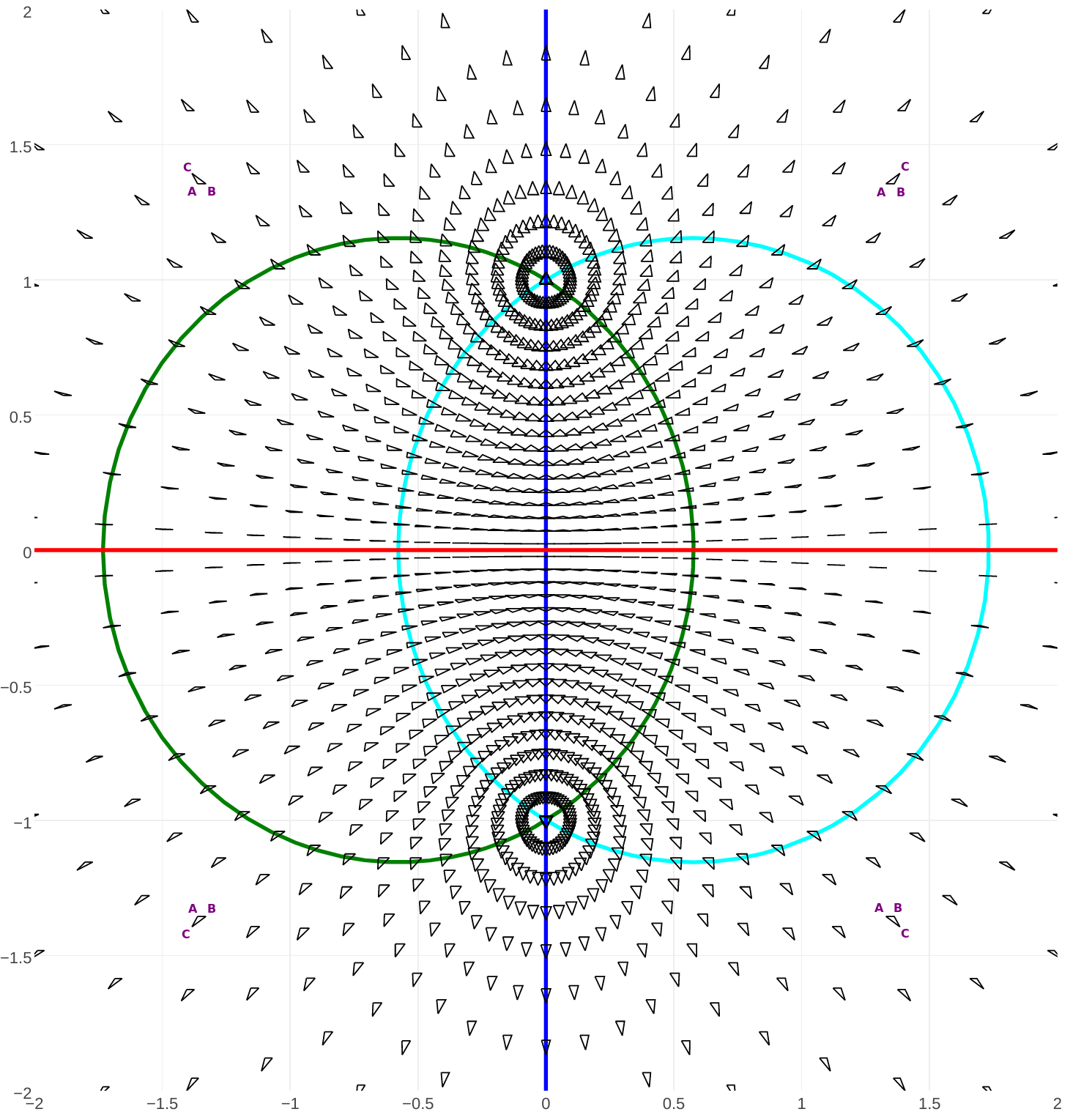
In the figure above, the red horizontal line is the set of flat triangles. The vertical blue line is that of triangles which are isoceles in $A_3$, while the green and cyan curves are respectively associated to $A_1$ and $A_2$.
As the semi-degenerate case $A_1=A_2$ corresponds to the point at infinity, the set of triangle shapes is homeomorphic to $\mathbb{C}\cup\{\infty\} \simeq \mathbb{S}^2$.
Most surprisingly, this correspondance is also geometric.
Theorem (Kendall, 1983): There exists a mapping $f$ from the set of triangles to the sphere of radius $1/2$ in $\mathbb{R}^3$ such that for all non-degenerate triangles $A$ and $B$ in $\mathbb{C}^3$,
$$ \text{d}_{L^2}([A],[B]) ~=~ \| f(A) -f(B)\|_{\mathbb{R}^3}. $$
Otherwise said, the Procustes distance defined in the section above is nothing but a chord distance on the sphere of triangles' shapes.
def chord( A, B ) :
"'Chord' distance between two triangles A and B."
a, b = normalize(A), normalize(B)
return (1 - mod2( herm(a,b) )).sqrt()
Exercise 1: Playing around with $A$ and $B$, convince yourself that the theorem above is true!
A = tensor([ [-1, 0], [ 1, 0], [ 0,0.] ])
B = tensor([ [ 1, 0], [-.5, np.sqrt(3)/2], [-.5,-np.sqrt(3)/2] ])
print("Chord distance : ", chord(A,B).item())
print(" on the sphere : ", np.sqrt(2)/2)
# 2D plot : the two triangles
plt.figure()
plot(A, "red")
plot(B, "blue")
plt.axis("equal")
plt.show()
# 3D plot : the Kendall sphere
M = KendallTriangles()
M.show()
M.show_pieces()
M.generate_spherical_sampled_data()
M.show_glyphs()
M.add_markers(A, "red" , "A")
M.add_markers(B, "blue", "B")
M.iplot('Kendall sphere')

C) A Riemannian shape space
Undoubtedly, we've understood something about the nonlinear space of triangles' shapes.
But we must go further: crucially, the chord distance is not a path distance. As it cannot be understood through infinitesimal "steps", it won't let us define any (proper) statistical model such as Gaussian laws, etc.
Fortunately, the associated arc distance on the sphere of triangles isn't difficult to compute either: if $a$ and $b$ are normalized transformations of $A$ and $B$, we can simply write
$$ \text{d}_{\text{arc}}([A],[B]) ~=~ \arccos(|a^\star b|). $$
N.B.: In the literature, the chord and the arc distance on a shape space are most often denoted by $\text{d}_F$ and $\rho$.
def arc( A, B ) :
"'Geodesic' distance between two triangles A and B."
a, b = normalize(A), normalize(B)
return mod( herm(a,b) ).acos()
Exercise 2: Playing around with $A$ and $B$, convince yourself that the formula above defines the intrinsic, Riemannian distance on the sphere of triangles.
A = tensor([ [-1, 0], [ 1, 0], [ 0,0.] ])
B = tensor([ [ 1, 0], [-.5, np.sqrt(3)/2], [-.5,-np.sqrt(3)/2] ])
print("Chord distance : ", chord(A,B).item())
print(" on the sphere : ", np.sqrt(2)/2)
print("Arc distance : ", arc(A,B).item())
print(" on the sphere : ", np.pi / 4)
# 2D plot : the two triangles
plt.figure()
plot(A, "red")
plot(B, "blue")
plt.axis("equal")
plt.show()
# 3D plot : the Kendall sphere
M = KendallTriangles()
M.show()
M.show_pieces()
M.generate_spherical_sampled_data()
M.show_glyphs()
M.add_markers(A, "red" , "A")
M.add_markers(B, "blue", "B")
M.iplot('Kendall sphere')
Most importantly, the arc distance is a geodesic path distance. In the next notebooks, we'll see how to generalize simple statistical operations to this convenient, homogeneous space. To conclude this introduction, let us finally mention a remarkable statistical result:
Theorem (Kendall, 1983): Let us draw our triangles' vertices according to an iid Gaussian law in the complex plane. Then, the resulting law on the quotient shape space only depends on the heigth coordinate.
If the aforementioned Gaussian law is isotropic, we retrieve the uniform density on the sphere. Otherwise, we observe a concentration of mass around the equator of flat triangles.
Exercise 3: Playing around with the code below, make sure that this is true!
M = KendallTriangles()
npoints = 1000000
s = 1.
points = s*random.randn(npoints,3) + 1j * random.randn(npoints,3)
M.set_data(points)
M.plot_data(N_triangles = 10, sigma = s)

M.clear_axis()
M.show_density(contours = True)
M.generate_spherical_sampled_data()
M.show_glyphs()
M.show_pieces()
M.iplot('Kendall sphere, ' + "{:.1e}".format(npoints) \
+ ' random triangles')