2) Statistical analysis on a shape space
%matplotlib inline
import matplotlib.pyplot as plt
import plotly
# run at the start of every notebook
plotly.offline.init_notebook_mode()
# Mandatory imports...
import numpy as np
from numpy import random
import torch
from torch import tensor
from torch.nn import Parameter
# Custom modules:
from kendall_triangles import KendallTriangles # Fancy visualization
from model import Model # Optimization blackbox
from display import plot # Simple plotting routine for triangles
# Finally, emulate complex numbers with pairs of floats:
from torch_complex import rot,normalize,herm,angle,mod2,mod,comp
A) Computing a Fréchet mean
In the previous notebook, we've seen that the set of triangles "up to similarities" can be endowed with a canonical, spherical metric structure. The arc (or geodesic) distance between two triangle shapes is given by:
def arc( A, B ) :
"'Geodesic' distance between two triangles A and B."
a, b = normalize(A), normalize(B)
return mod( herm(a,b) ).acos()
We now implement some (simple) statistical operations in this nonlinear space. Our key message: the standard statistician's toolbox can be generalized to Riemannian manifolds, both from a theoretical and a practical point of view.
First, let us generate some arbitrary population of shapes:
N = 100
A_k = torch.stack((
.05*torch.randn(100,2)+tensor([-.5,-.5]),
.05*torch.randn(100,2)+tensor([+.5,0. ]),
.50*torch.randn(100,2)+tensor([ 0., 1.]),
), 1) + 3*torch.randn(100,1,2)
And display it in the 2D plane:
plt.figure()
plot(A_k[:20], "green")
plt.axis("equal")
plt.show()

In the shape space:
M = KendallTriangles()
M.add_markers(A_k, "green", "A_k", .5)
M.generate_spherical_sampled_data()
M.show()
M.show_glyphs()
M.show_pieces()
M.iplot('Our triangles on the Kendall sphere')
Given such an empirical distribution $A_k$, what it the simplest statistic that we could compute? The mean, obviously. But beware: on a sphere, there is no such thing as a "$+$" operator.
One of the most sensible ways of generalizing the mean to an arbitrary metric space $(X,\text{d})$ is the least-square definition. For any order $p>0$, we thus define the $p$-Fréchet mean of the $A_k$'s through:
$$ F_p(A_1,\dots,A_N) ~=~ \arg\min_{x\in X} \,\sum_{k=1}^N \text{d}(x,A_k)^p $$
Exercise 1: Show that in a Euclidean vector space, the Fréchet means of order 1 and 2 respectively coincide with the median and the arithmetic mean of the distribution.
class FrechetMean(Model) :
"Find the Frechet mean of a population of polygons."
def __init__(self, guess, p=2) :
"Defines an initial guess and the Frechet exponent."
super(Model, self).__init__()
self.x = Parameter(guess)
self.p = p
def __call__(self) :
"Returns the current guess."
return self.x
def cost(self, targets) :
"Returns the mean p-distance to the current guess."
return ( arc(targets, self())**self.p ).mean()
Using PyTorch, computing a Fréchet mean is that simple:
# Initial guess: any non-degenerate triangle should be ok
A0 = tensor([ [-1.,0.], [1.,0.], [0.,1.] ])
# Frechet means of order 1 and 2
FMedian = FrechetMean( A0, p=1 )
FMean = FrechetMean( A0, p=2 )
FMedian.fit( A_k )
FMean.fit( A_k )
# For a clean display, let's normalize everybody
median = normalize( FMedian())
mean = normalize( FMean() )
a_k = normalize( A_k )
Without aligning the shapes onto a reference mean, displaying the population is not easy:
plt.figure()
plot( a_k[:10] , "green")
plot( mean, "red")
plot( median, "blue")
plt.axis("equal")
plt.show()

Thankfully, the Kendall sphere lets us check that our computations are correct:
M = KendallTriangles()
M.add_markers(a_k, "green", "A_k", .5)
M.add_markers(mean, "red", "mean")
M.add_markers(median, "blue", "median")
M.generate_spherical_sampled_data()
M.show()
M.show_glyphs()
M.show_pieces()
M.iplot('Mean and Median of our population')
Exercise 2: What's the difference between using a mean and a median?
B) Computing a geodesic
Under mild technical assumptions, Riemannian manifolds let us define geodesic curves through an order 2 ODE. If $a$ and $b$ are two points in the manifold, and if $v$ is some tangent vector at location $a$, $\text{Exp}_a(v)$ will denote the position at time $t=1$ of the unique geodesic curve $\gamma_t$ such that
$$ \gamma_0 ~=~a ~~~~~\text{and}~~~~~ \dot{\gamma}_0~=~v. $$
The length of such a geodesic curve is simply equal to the norm of the tangent vector $v$ at position $a$.
A standard result of Riemannian geometry is that for any reference point $a$, such an Exponential map defines an isomorphism from a neighborhood of $0$ (on the tangent plane) to a neighborhood of $a$ (on the manifold).
We can thus define the $\text{Log}_a$ map as the inverse of $\text{Exp}_a$ in a neighborhood of $a$, and use it to represent the curved manifold in the tangent vector space:
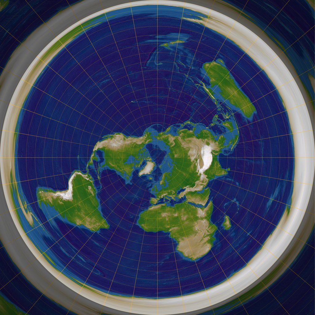 Exponential chart of the Earth, at the North pole. Image from Wikipedia, by RokerHRO.
Most often, the $\text{Exp}$ and $\text{Log}$ operators are tedious to implement. But in the very specific (and important!) case of polygonal shapes up to similarities, the classic Kendall theory provides us with the following formulas:
def log(a,b):
"""
Assuming that a and b are both normalized, returns
the Riemannian logarithm of b at point a.
"""
# Optimally rotate b onto a
bsa = herm(b, a)
b = rot(b, angle(bsa))
# Compute the normal vector
c = b - (a*b).sum()*a
c = c / (c**2).sum().sqrt()
L = arc(a,b)
return L*c
def exp(a,v):
"Shoots along the tangent vector v at location a."
L = (v**2).sum().sqrt()
return a*torch.cos(L) + (v/L)*torch.sin(L)
def geodesic(a,b):
"""
Returns the geodesic between two *normalized* polygons a and b,
sampled on 10 timesteps with the normal tangent vector at a.
"""
v = log(a,b)
g_t = [ exp(a, t*v) \
for t in torch.linspace(0,1,11) ]
return torch.stack( g_t )
Exercise 3: Please convince yourself that it works!
# Compute an arbitrary geodesic segment
a = a_k[1]
g = geodesic(mean, a)
# Display on the phere
M = KendallTriangles()
M.add_markers(g, "green", "geodesic", .5)
M.add_markers(mean, "red", "mean")
M.add_markers(a, "blue", "target")
M.generate_spherical_sampled_data()
M.show()
M.show_glyphs()
M.show_pieces()
M.iplot('An arbitrary geodesic')
C) Tangent PCA
We've seen how to compute a mean, and how to map our manifold data on a tangent vector space. The next step: analyse the variability in a neighborhood of the mean through a standard, linear statistical analysis.
Exercise 4: Perform PCA in the tangent plane at the mean's location. How many modes do we need to represent the data? Is this a surprise?
Hint: Please use the sklearn.decomposition.PCA module.
## Insert your code here.
# Compute the log-map of the A_k's around the mean
v_k = torch.stack( [ log(mean, a) for a in a_k ] )
# Turn it into an N-by-6 tensor...
v_k = v_k.view(len(v_k),-1)
v_k = v_k.detach().cpu().numpy()
# That we can feed to scikit-learn's PCA module
from sklearn.decomposition import PCA
pca = PCA()
V_k = pca.fit_transform(v_k)
print("Explained variance: ")
print(pca.explained_variance_)
run -i nt_solutions/Kendall_2/exo4
Exercise 5: Display the two principal modes of variation on the Kendall sphere. Is this method accurate enough?
Hint: Use the inverse_transform method of scikit-learn's PCA module.
## Insert your code here.
# We only need the first two features...
pca = PCA(n_components=2)
V_k = pca.fit_transform(v_k)
sig = np.sqrt(pca.explained_variance_)
# Let's retrieve the two directions:
mode_1 = tensor( sig[0]*pca.inverse_transform( [1.,0.] ))
mode_2 = tensor( sig[1]*pca.inverse_transform( [0.,1.] ))
mode_1, mode_2 = mode_1.float().view(3,2), mode_2.float().view(3,2)
# Fancy display
M = KendallTriangles()
M.add_markers(a_k, "green", "A_k", .5)
M.add_markers(mean, "red", "mean")
M.add_markers(exp(mean, mode_1), "blue", "+e_1")
M.add_markers(exp(mean,-mode_1), "blue", "-e_1")
M.add_markers(exp(mean, mode_2), "cyan", "+e_2")
M.add_markers(exp(mean,-mode_2), "cyan", "-e_2")
M.generate_spherical_sampled_data()
M.show()
M.show_glyphs()
M.show_pieces()
M.iplot('The principal modes of variation')
run -i nt_solutions/Kendall_2/exo5
Exercise 6: Display the population as seen through the log-mapping at the mean's location. Is this a faithful representation of the dataset's geometry?
## Insert your code here.
run -i nt_solutions/Kendall_2/exo6
plt.figure(figsize=(10,10))
plt.scatter(V_k[:,0], V_k[:,1], color="green")
plt.scatter( [0.], [0.], color="red", s=125)
plt.scatter( [sig[0],-sig[0]], [0.,0.], color="blue", s=81)
plt.scatter( [0.,0.], [sig[1],-sig[1]], color="cyan", s=81)
midway = plt.Circle((0,0),np.pi/4,color='r', fill=False)
plt.gcf().gca().add_artist(midway)
cut_locus = plt.Circle((0,0), np.pi/2,color='r', fill=False)
plt.gcf().gca().add_artist(cut_locus)
plt.axis("equal")
plt.axis([-np.pi/2,np.pi/2,-np.pi/2,np.pi/2])
plt.title("Exponential chart at the mean location")
plt.show()
